Overview of directed graph editing
 Caution Caution <dot> syntax is not compatible with versions of TWiki:Extensions.WysiwygPlugin prior to 28 June 2009. It is recommended that you upgrade WysiwygPlugin if you are running an older version. If that is not practical then raw editing is recommended, or use <sticky> tags to protect the dot tags. prior to 28 June 2009. It is recommended that you upgrade WysiwygPlugin if you are running an older version. If that is not practical then raw editing is recommended, or use <sticky> tags to protect the dot tags. |
Introduction
Support for creating advanced directed graphs has been installed on this TWiki installation. Directed graphs are rendered by
Graphviz
. Only the most important basics are covered here, you should consult the dotguide.pdf from Graphviz's homepage for a more thorough guide on creating directed graphs.
What are directed graphs?
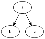
The graph:

|
To the left here you can see a simple directed graph with three "nodes", one on the top and two below (which are connected from top to bottom). Connecting these nodes you can also see two "edges", which is the technical term for the arrow connecting the three nodes.
When entering directed graphs in TWiki, everything you do is to define nodes and their edges (or connections); the directed graph engine then does all placing by itself, fully automatic.
No layout more than which nodes and their relationship, together with node and edge style is defined by the author; the engine takes care of all layout and placing of nodes, which makes creating advanced graphs extremely simple and fast.
Using more advanced syntax very advanced graphs can be created, including subgraphs and balanced trees and record graphs. This document only focusses on "normal" directed graphs; if you want to experiment more with the graph engine, consult the dotguide on www.graphviz.org.
|
Examples
A simple graph with two nodes
The graph:

|
The code:
<dot file="simple_two_nodes" dothash="off">
digraph G {
 a -> b;
}
</dot>
|
Explanation:
In order to describe a graph you start by typing:
<dot>
digraph G {
After the curly opening bracket ({) the actual graph description is located. When you have defined your graph you close it by typing:
}
</dot>
Inside those two parts you place your graph description. You can define nodes and edges (connection between nodes); you define edges by typing "node1" -> "node2"; which also implicit defines both nodes node1 and node2. If the nodes' names doesn't contain spaces or other special characters, the quotation marks can be ignored.
As you can see in this example we actually only define exactly one edge, the link between node a and node b, by typing a -> b;. Note also how the line is terminated by a semi-colon (;).
|
Added attributes to nodes and edges
The graph:

|
The code:
<dot file="added_attributes" dothash="off">
digraph G {
 a [style=filled, color=green];
 b [style=filled, color=red];

 a -> b [style=dotted, color=blue];
}
</dot>
|
Explanation:
This example is very similar to the above example, with the difference that we have defined some attributes to both the nodes and the edge. As you can see the nodes are filled with green and red, respective. The edge has been changed to have a dotted line instead of a solid line.
If you want to assign attributes to nodes, the nodes have to be defined first, which means they appear on a line on their own. The order of node and edge definitions is not important, the whole file is parsed before any layout is begun.
The first line in the graph a [style=filled, color=green]; defines the node a and assigns the attributes style=filled and color=green. These two attributes make the node filled with the color green.
|
As you can see to assign attributes to a node you just type its name (with the optional quotation marks) followed by the attribute definitions separated by commas, as it appears in the example above.
To add attributes to edges (i.e. arrows) just add the attributes to the line of the edge definition as can be seen on the last line of the graph definition.
Adding labels to edges
The graph:

|
The code:
<dot file="with_labels" dothash="off">
digraph G {
 a -> b [label="link"];
}
</dot>
|
Explanation:
Edges can be labelled by adding the attribute label="text" at the edge definition, as can be seen in the code of this example.
|
Adding subgraphs
The graph:

|
The code:
<dot file="add_subgraphs" dothash="off" >
digraph G {
  a -> b;
  a -> c;

  subgraph cluster0 {
    node [style=filled, color=white];
    style=filled;
    color=lightgrey;
    rank=same;
    b;
    c;
  }

  c -> d;
  b -> d;
}
</dot>
|
Explanation:
If you want to group nodes together, you put the node definitions inside a subgraph clusterXXX { } statement.
Note: the name of the subgraph must begin with cluster.
The subgraph has the attributes style=filled and color=lightgrey which makes the subgraph filled with the color light grey. The subgraph also has the attribute rank=same which makes all nodes defined inside the subgraph appear on the same level (i.e. they have the same rank).
You can also see the nodes b and c are defined in the subgraph by the last two lines in the subgraph.
All nodes defined in the subgraph have the attributes style=filled, color=white by adding the line node [style=filled, color=white];.
|
Grouping nodes
The graph:

|
The code:
<dot file="grouping_nodes" dothash="off" >

digraph G {
  {
    node [shape=plaintext, fontsize=16];

    1975 -> 1980 -> 1985;
  }

  { rank=same; 1975; a; b; c; }
  { rank=same; 1980; d; e; }
  { rank=same; 1985; f; g; h; i; }

  a -> d;
  b -> e;
  c -> e;
  d -> f;
  e -> g;
  e -> h;
  e -> i;
}
</dot>
|
Explanation:
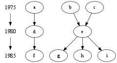
In this graph three groups are defined, by putting them inside a block, defined by { }.
The first group defines the nodes 1975, 1980 and 1985, by connecting them together; these nodes are of the type "plaintext" with font size equal to 16. We do this because the years are to be placed to the left as a timeline and therefore the font size is choosen to be a little larger.
The next three groups for example { rank=same; 1975; a; b; } ensures that the nodes 1975, a and b are on the same level, of course, because a and b occured in 1975 (It is left as an exercise to the reader to figure out what a and b actually is).
Following the last group definition we define all edges.
|
Ladder Diagrams
The graph:

|
The code:
<dot map=1>
digraph ladder {  ranksep=".1"; nodesep=".1";

# Define the defaults
  node [shape=point fontsize=10]
  edge [dir=none fontsize=10]

# Define the top nodes
  left [shape=none]
  right [shape=none]

# Column labels
  a [shape=none]
  b [shape=none]
  c [shape=none]
  d [shape=none]

# Leftmost vertical column
  left -> a [style=invis]  a -> a1 [style=invis]
  a1 -> a2 -> a3 -> a4 -> a5 -> a6 -> a7 -> a8 -> a9 -> a10 ->
    a11 -> a12 -> a13 [weight=1000]

# Rightmost vertical column
  right -> d [style=invis]   d -> d1 [style = invis]
  d1 -> d2 -> d3 -> d4 -> d5 -> d6 -> d7 -> d8 -> d9 -> d10 ->
    d11 -> d12 -> d13 [weight=1000]

# Draw the top labels with the dotted line
  { rank=same; left right
    left -> right [style=dotted]  }

# Draw the 4 column headings, no line
  { rank=same;
    edge[style=invis]
    a -> b -> c -> d   }

# Draw the two center columns
  b1 -> b2 -> b3 -> b4 -> b5 -> b6 -> b7 -> b8 -> b9 -> b10
  c1 -> c2 -> c3 -> c4 -> c5 -> c6 -> c7 -> c8 -> c9 -> c10

# Now each step in the ladder
  { rank=same;
    a2 -> b2 [dir=forward label="S1" URL="http://twiki.org/" ]  }
  { rank=same;
    b3 -> c3 [dir=forward label="S2" ]  }
  { rank=same;
    c4 -> d4 [dir=forward label="A"]  }
  { rank=same;
    c5 -> d5 [dir=back label="B"]  }
  { rank=same;
    b6 -> c6 [dir=back label="C"]  }
  { rank=same;
    a7 -> b7 [dir=back label="D"]  }
  { rank=same;
    a8 -> b8 [dir=forward label="E"]  }
  { rank=same;
    a9 -> b9 [dir=back label="F"]
    b9 -> c9 [dir=forward label="G"]  }
  { rank=same;
    a10 -> b10 [dir=back label="H"]  }
  { rank=same;
    a11 -> d11 [dir=forward label="I"]  }
  { rank=same;
    a12 -> d12 [style=dashed dir=both label="J"]  }
}
</dot>
|
Explanation:
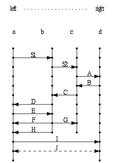
The ladder diagram uses the weight operand to force straight edges. The heaver the weight, the edge will be shorter, straighter, and closer to vertical.
Defaults are established using dir=none for the edges. This causes the edge lines to be undirected, and are drawn without an arrow.
The edges of the top two rows specify style=invisible. This keeps the columns aligned, but omits drawing any lines.
Each horizontal "rung" in the ladder is kept on the same level by specifying rank=same
|
Node types
Choose the shape of a node by adding the attribute
shape to the node definition.

box
|

polygon
|

ellipse
|

circle
|

point
|

egg
|

triangle
|

plaintext
|

diamond
|

trapezium
|

parallelogram
|

house
|

hexagon
|

octagon
|

doublecircle
|

doubleoctagon
|

tripleoctagon
|

invtriangle
|

invtrapezium
|

invhouse
|

Mdiamond
|

Msquare
|

Mcircle
|
Arrow types
The form of the edge can be set by using the
arrowtail and
arrowhead attributes with edges. The attribute
arrowtail sets the shape of the arrow at the source node, while
arrowhead sets the shape of the arrow at the destination node.

normal
|

dot
|

odot
|

inv
|

invdot
|

invodot
|

none
|
--
TWiki:Main.MikaelOlenfalk
- 08 Aug 2005
 TWiki Web>Plugins>DirectedGraphPlugin>HowtoDirectedGraphs (2024-03-02, TWikiAdminUser)
 EditAttach